Intro

Not too long ago image classification was found to be a difficult and unwieldy task for many of the novel machine learning algorithms. However, the entire field witnessed the astounding ground-breaking accomplishment made by Alex Krizhevsky when he submitted his Convolutional Neural Network (CNN) to the ImageNet Large Scale Visual Recognition Challenge in 2012 which won with a 15.3% error rate over the second place competitor with an error rate of 26.2%. Following his jaw-dropping performance, CNNs have become the engine that drives every achievement we see in computer vision research.

Despite CNNs becoming the mainstream machine vision algorithm to use after Alex Krizhevsky made AlexNet, they were actually invented all the way back in 1994 when Yann LeCun made LeNet5. However, LeNet5 was unable to utilize the resources in a GPU the way AlexNet did, which is the reason why AlexNet has a deeper network and can train quicker than LeNet5. As a result, Alex Krizhevsky transformed the world by showing the true power of a CNN when it is able to capitalize on more efficient hardware.

At first it may seem like CNNs are complicated to create and train, but thanks to some high level libraries such as PyTorch and TensorFlow along with Python make the design process a breeze. Below I will be using Keras, a library designed to be used with TensorFlow, and Python to demonstrate how to make some of the different layers and how to adjust different parameters.

Convolutions

What makes a convolutional neural network differ from a neural network is due to their use of convolutions. A way to think of a convolution is they are primarily used to find how similar a filter is to an area of an image. This is not exactly what convolutions accomplish, and can be more accurately described as a process that picks up a signal in images. The signal it picks up is commonly known as a feature, and can be something as simple as a horizontal line.

The math behind convolving a filter and an area of an image is pretty simple. Typically you shouldn’t use 5x5 or 7x7 filters in your CNN architecture since VGGNet and ResNet among others showed you don’t need anything larger than a 3x3 filter. That being said, the process of convolving a 3x3 filter with an image begins by taking a 3x3 area of the image (for example, the top left) and multiplying each value in the image segment with the corresponding position in the filter. Once the you get the nine multiplied numbers, you add them all up to get one final value which is known as an activation.

The equation above shows a mathematical representation of finding an activation between a filter, $f$, and an image segment, $img$, by convolving the two together. In the 3x3 filter example, $f_w$ would be equal to the width of the filter and $f_h$ would be the height which are both equal to 3.

After you find the activation of one filter for one area of the image, you convolve your filter with a new 3x3 area of the image to produce a new activation value. This is done by starting in one area of the image, say the top left, and moving the filter across the image, say left to right and then top to bottom, to find the actions of every area of the image. If you are working with a 32x32 image and you follow the process I just described, you should end up with 30x30 activations which will become what is know as the activation map.

In order to add power to the CNN you may be building, you would obviously want more than just a single convolution in a layer. That is, you wouldn’t want only one filter that finds signals for horizontal lines, but you would want multiple filters to find other features such as vertical lines, diagonal lines, curved lines, and many other features found in your image. To do this, you simply stack several filters together which will produce a 3-dimensional activation map. For example, if the first layer of a CNN contains 64 filters and you apply 3x3 convolutions to a 32x32 image by following the same approach as above, you would end up with a 30x30x64 3-dimensional matrix, otherwise known as a tensor.

One way to alter a convolution layer is by adjusting what is known as the stride. When the filter slides across the image, it does not have to visit every segment of the image. Instead, it can jump across certain pixels by the amount the stride is set at. In the example above we were working with a 32x32 image to create an activation map of 30x30 which used a stride value of 1. When you increase the stride value to 2, you would start at the top left of the image as normal, then you would move two pixels over instead of just one which would cut down on the number of activations in each dimension by 2, producing a 15x15 activation map. You may lose some data while increasing the stride value, but the CNN will in turn be able to train quicker since it will need less time to compute.

Another common parameter to tweak on a convolution layer is the padding. Sometimes a CNN architecture may benefit by producing a 32x32 activation map when given a 32x32 image, but in order to do this they need to increase the padding. In order to get a 32x32 activation map, the image can be padded with 0s along the outer border. With the outer ring full of 0s, the filter can begin to make the activation map centered over the top left pixel.

I’ve been describing the convolution layer as a way to find signals in the original image, but the convolution layer can use all of the aforementioned techniques on previous activation maps made by other layers. If you think about it, the original image is more than likely a 32x32x3 image, where the additional dimension come from the three RGB channels. That means the image is a 3-dimensional tensor just like the stacked activation maps. Building up convolutional layers is where CNNs get their description of being “deep-learning”.

The real power of CNNs shines by stacking convolution layers on top of each other. At the early convolution layers, filters will activate when seeing simple shapes, such as lines. However, once you start to get deeper into the network, the convolution layers piece together the lines from previous layers to recognize higher-level features such as faces or honeycomb type structures.

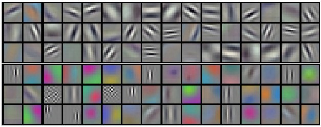
The 96 filters in the first convolution layer of AlexNet. Each filter is 11x11x3.

Writing a convolution layer in Keras can be written in one line. The library takes care of all the math and GPU support the CNN may need. If you are making the initial convolution layer, you will need to specify the input_shape parameter, otherwise Keras is able to figure out the input_shape for the preceding layers. For example, here is how you could write the first convolution layer for a 32x32x3 image with 16 3x3 filters, a stride of 1, and a padding of zeros around the edge:

keras.layers.Conv2D(16, kernel_size=(3, 3), strides=(1, 1),
                 activation='relu', padding='same',
                 input_shape=(32, 32, 3))

Layers

The convolution layer gives convolutional neural networks a cutting edge over neural networks when it comes to image analysis, but there are still more layers CNNs regularly utilize to increase the performance of the model. When it comes to speed, many CNNs use pooling to reduce computational needs. In addition to pooling techniques, CNNs may also use a technique called dropout to reduce some of the bias the model may receive while training.

Pooling

The idea behind pooling layers is simple, but their application has proven to be quite useful in reducing the dimensionality and complexity of a CNN. This reduction has even shown to help with overfitting due to eliminating many of the parameters in a previous layer. The pooling layer works by reducing an area of an image down to a single value, typically by averaging the numbers in an area or finding the max value. A pooling layer will most commonly be designed with a 2x2 filter with a stride of 2, which allows the pooling layer to look at a previous activation map and cut down each dimension in half. For example, using a 2x2 pooling filter with a stride of 2 on an activation map with size 50x50x100, will result in a new tensor of size 25x25x100, since the pooling layer only affects the dimensions of each activation map.

There are many arguments to whether you should use average pooling or max pooling, but average pooling has recently fallen out of practice due to max pooling being shown to work better in practice. However, average pooling may still be useful towards the end of your network near the fully-connected layers.

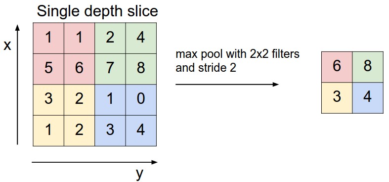
An example of max pooling being used with a 2x2 filter and a stride of 2. The dimensionality of the matrix on the left is reduced from 4x4 to 2x2 on the right.

When designing a CNN you typically place a pooling layer between two convolution layers. Writing this in Keras is once again a simple task. Following the code from above, you can place the pooling layer right after the first convolution layer and specify the pool_size and strides parameters. The pool_size parameter refers to the filter size of the pooling layer. The example below is an incomplete representation of the model used in a Keras tutorial adopted to follow the code above.

model = Sequential()
model.add(keras.layers.Conv2D(16, kernel_size=(3, 3), strides=(1, 1),
                 activation='relu', padding='same',
                 input_shape=(32, 32, 3)))
model.add(keras.layers.MaxPooling2D(pool_size=(2, 2), strides=(2, 2)))
model.add(keras.layers.Conv2D(32, (3, 3), activation='relu'))

Dropout

When a model is able to perform very well on a training set, but is unable to keep the same pace in practice, the model is more than likely experiencing a phenomenon know as overfitting. The problem of overfitting in CNNs can stem from the over-dependence on certain features, or activations. To combat this problem, a CNN architecture may include a dropout layer which randomly selects activations and sets them to 0.

You can use dropout pretty much anywhere in your CNN architecture, and below I will use a dropout layer right before the second convolution layer. The dropout layer only requires the rate parameter to be specified, which is the chance each activation will be randomly set to 0.

model = Sequential()
model.add(keras.layers.Conv2D(16, kernel_size=(3, 3), strides=(1, 1),
                 activation='relu', padding='same',
                 input_shape=(32, 32, 3)))
model.add(keras.layers.MaxPooling2D(pool_size=(2, 2), strides=(2, 2)))
model.add(keras.layers.Dropout(0.2))
model.add(keras.layers.Conv2D(32, (3, 3), activation='relu'))

Fully-Connected

Used in regular neural networks, fully-connected layers have neurons which are fully connected to all the activations in the previous layer. They are typically found just at the end of the network and are used as the last layer that decides the output. In Keras, fully-connected is referred to as a dense layer, and takes in the parameters units and activation. The units parameter will be the number of output units, where the activation will likely remain "relu" unless it is the final layer in which case it should be "softmax". The following finishes off the architecture of the CNN built thoughout this blog. It incorporates fully-connected layers as well as a flattening of the final activation map. The Flatten() function simply turns a 3-dimensional tensor into a 1-dimensional fully-connected layer. The final dense layer will output to 10 classes, in the case you have a classifier that is deciding between ten classes.

model = Sequential()
model.add(keras.layers.Conv2D(16, kernel_size=(3, 3), strides=(1, 1),
                 activation='relu', padding='same',
                 input_shape=(32, 32, 3)))
model.add(keras.layers.MaxPooling2D(pool_size=(2, 2), strides=(2, 2)))
model.add(keras.layers.Dropout(0.2))
model.add(keras.layers.Conv2D(32, (3, 3), activation='relu'))
model.add(keras.layers.MaxPooling2D(pool_size=(2, 2), strides=(2, 2)))
model.add(keras.layers.Flatten())
model.add(keras.layers.Dense(1000, activation='relu'))
model.add(keras.layers.Dense(10, activation='softmax'))

Conclusion

Although image analysis can seem like a daunting task, the recent work on CNNs has allowed the entire machine vision field to blossom in a very fruitful manner. Ever since the work of AlexNet, we have seen many improvements to CNNs over the years as well as powerful, yet simple tools and libraries to handle it. In particular, Keras allows programmers to easily construct their own CNN architecture, and train in relatively no time at all.